Introduction

Overview

Teaching: 20 min
Exercises: 30 min

Questions

• How do I start working in Galaxy?

• What does my raw sequencing data looks like?

• Do I have good enough quality and sequencing depth for my assembly?

Objectives

• Getting familiar with Galaxy’s workflow and history

• Understand the data generated and make a decision on how to process MinION data

Introduction

For the bioinformatics analysis of your genomes, we will be working in Galaxy.

There are two main online galaxy platforms; the global server: https://usegalaxy.org/ and the European server: https://usegalaxy.eu/. The global version has a slightly larger set of programs than the European version. However, the European version runs in general slightly faster, and therefore you are recommended to use the European server.

Overview of Genome Assembly Processes

Next-generation Sequencing (NGS) generates DNA reads in parallel, which are massive amount of short sequences of nucleotides. The length of these reads depends on the sequencing platforms as well as the methods used for extracting the DNA. Short-read NGS platform such as Illumina generate an average read length of 2 x 150 bp to 2 x 300 bp with high accuracy. In the past decade, long-read sequencing have become a reality, with the two leading platform are PacBio and Oxford Nanopore Technologies. Current PacBio HiFi can generate up to 25kb reads with high accuracy, while Nanopore can generate ultra long reads (>900 kb) but with less accuracy.

Long-read sequencing are crucial to solve assembly of complex genomic regions such as repeats, something that short-read could not achieve. A hybrid assembly (combining both the accuracy of short-reads and with long-reads to connect fragments) are used to generate a complete, high-quality genome. Nevertheless, the field is moving rapidly, opening a new avenues to look at microbial diversity at strain-level resolutions.

Because Nanopore sequencing results in so much longer reads, different bioinformatics tools need to be applied to process the data, as compared to the data generated by Illumina sequencing. Therefore, be careful to use bioinformatics programs, which are applicable for short or long reads depending on the dataset you have. In this course we are solely working with Nanopore sequencing.

More information on sequencing techniques:

• https://www.nature.com/articles/nrg.2016.49
• https://www.ncbi.nlm.nih.gov/pmc/articles/PMC6020069/

Ryan Wick provides a nice “Guide to bacterial genome assembly” as a starting point to choose which approaches and techniques to assemble your genome. He also write an approach in combining ONT long reads with Illumina short reads to achieve perfect assemblies: Assembling the perfect bacterial genome using Oxford Nanopore and Illumina sequencing.

The general pipeline for processing nanopore reads into whole genomes are:

1. Trimming and filtering reads
2. Assembly of the reads into a genome
3. Polishing the assembly
4. Analysing the genome

We will be using similar pipeline to the one suggested by Ryan Wick with several measures to check quality in between each steps.

Importing Data into Galaxy

There are several ways we can input our data into Galaxy. We can upload datasets from our local machine, fetch from a public repository such as Zenodo, or reuse data from Galaxy history.

We will inform you how to fetch your raw sequencing data when it is ready. In the meantime, we can do an exercise using the data from previous year (2022), which are available from Zenodo. We will be using the strain with decent reads (barcode02).

Let’s login to Galaxy and import this data into our history:

1. Go to https://usegalaxy.eu/
2. Click Login or Register. Create an account and activate (if you hadn’t so)
3. Import the data by pressing the Upload Data button on the upper right corner and choose the Paste/Fetch data button at the bottom window.
4. Change the name from New file to barcode02.fastq.gz and paste the zenodo link: https://zenodo.org/record/6475902/files/barcode02.fastq.gz into the box.
5. Press start to download

Discussion 01

Each item in the Zenodo repository are the sample raw reads that has been demultiplexed (one strain each).

1. How many gigabytes of data are there?
2. How much data was generated for an average sample?
3. Why do we have uneven distribution of data for each samples?
4. What kind of information can you get from a FASTQ file? What are the differences with a FASTA format?

Solution

TBD

1. There are two main data formats which are relevant for your bioinformatics analysis. The first format is called FASTQ. It is usually used to store the raw reads (that is the nucleotide sequence string) together with their estimated quality(represented as ASCII bytes – not part of the curriculum). Data in fastq format can be identified by the endings: *.fq or *.fastq. The other format is called fasta. It is used to store any sort of DNA or amino acid sequence. Data in fasta format can be identified by the endings: *.fasta, *.fa, *.fna, *.fas or *.fsa. To save storage space data files are often compressed. Most often used is a Gzip compression, which results in an added *.gz at the end of the file name for example: example.fq.gz or example.fa.gz. When uploading files to galaxy, files get automatically unzipped, so this should not be an issue.

Importing and editing a published workflow

We have prepared a template workflow that you can edit and use in your genome assembly and annotation. The template workflow are split into different steps with several measures for checking the quality in between steps.

Let’s start by importing and exploring an initial QC workflow:

1. In a new tab, open this link: https://usegalaxy.eu/u/matinnu/w/01rawqc
2. On the top-right corner, click the + button (import workflow)
3. Click start using this workflow
4. Click on the name of the newly imported workflow (imported: 01_Raw_QC) and click Edit
5. Explore the workflow and make changes if necessary

Discussion 02

1. What is the input and final output of the workflow?
2. What are the purpose of the two main tools in the workflow?
3. Do you think Kraken2 is suited for long-read sequences?

Solution

TBD

When you are contempt with the workflow, click save. Next, we will run the analysis on barcode02.fastq (the smallest dataset).

1. Click the “play” button on the top-right corner (Run Workflow)
2. If the workflow does not show in detailed view, click Expand to full workflow form
3. Set Send results to a new history to yes.
4. Change the history name to “01_Raw_QC_2021_sample02”.
5. On the 1: input dataset, select 2: barcode02.fastq as the input.
6. Click Run Workflow on the top panel.

Working with Galaxy history

In Galaxy, each analysis will run on different history. You can have multiple history and switch between history depending on your needs.

We just run a simple QC to our raw reads, and it might take a while for the jobs to finish. Note that we have made some of the intermediate jobs hidden.

Discussion 03

When the job is done, let’s look at the output of the jobs in the history. Open the Nanoplot result by clicking the “eye” (view data) icon.

1. Find out the value of these parameters:
   • Total base
   • N50
   • Mean / Median Length
   • Mean / Median Quality
   • Your longest read
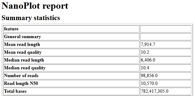
2. Note that this sample have 506.4 MB (Mega Bytes) of data and a 262.4 MBp (Mega Base Pairs) of reads. Which one is more appropriate to measure the sequencing yield?
3. What does N50 means? What is a good N50 value?
4. There are 66% of reads that are above Q10. What does this mean? What is a Q-score?
5. Do you think you have enough data for the assembly? What sequencing depth do you expect? How do you calculate a sequencing depth?

Solution

Example of Nanoplot result

Before the assembly a quality check is necessary. For that we can use Nanoplot with default settings. Nanoplot gives several output files, but you can get an easy overview with the HTML report. The most important numbers there the mean read quality and the read length N50. The read quality is denoted as a Phred score and is for nanopore reads typicall not very high. Anything above 7 should be fine. If you want to know more, it is possible to calculate back from the Phred score to the estimated probability of erroneous base pairs. The N50 is a measurement for the contiguity or the mean read/contig length. It is defined as the sequence length of the shortest contig at 50% of the total genome length. Low N50 (<1000bp) of the nanopore reads usually indicate sheared DNA, which can occur due to problems during the library prep or DNA extraction.

Let’s open the Krona Pie Chart to visualize the Kraken2 result.

1. What does Kraken2 says about the majority of the reads? What species are assigned?
2. Do you see potential contamination in your reads?
3. Would you trust Kraken2 result as the taxonomic placement of your assembly or do you want to try another approach? Which database are being used by Krona for the taxonomic assignment?

Solution

TBD

Concluding the QC Analysis

Based on the QC, we have good quality and sufficient amount of reads for the assembly. Nevertheless, we might improve our assembly by filtering out the shorter reads (and perhaps bad quality reads?), which we will do in the next steps.

Key Points

• You can start working in Galaxy by getting familiar to importing data, using history, and manipulating workflows.

• Tools such as Nanoplot and Kraken2 can give you information about the quantity (yield), quality (Q-score, N50, and read distribution), and possible contamination.

• QC are valuable to decide how the assembly process should be approached. It can tell us whether more sequencing data need to be generated or a certain part of the data need to be filtered. Overall, the decision might be a case by case basis.

Filtering and Assembly

Overview

Teaching: 20 min
Exercises: 30 min

Questions

• How do I assemble my genome?

• How do I asses my assembly result?

Objectives

• Getting familiar with assembly tools and use them to assemble a genome

Switching history & using template workflow

If you cannot find 27255_raw_2021 history, you can also reuse other histories that already has the barcode02.fastq.gz data.

We will go back to use the raw data from the 27255_raw_2021 history to assemble the sample file barcode02.fastq:

1. On the history panel, click the second icon from the left (view all histories)
2. Find the 27255_raw_2021 history which contains the raw read data, and click Switch to. Note that the history will move to the left as the Current History.

We have prepared the next workflow for you:

1. In a new tab, open this link: https://usegalaxy.eu/u/matinnu/w/02assembly
2. On the top-right corner, click the + button (import workflow)
3. Click start using this workflow
4. Click on the name of the newly imported workflow (imported: 02_Assembly) and click Edit
5. Explore the workflow and make changes if necessary

Running the workflow

When you are contempt with the workflow, run it by:

1. Click the “play” button on the top-right corner (Run Workflow)
2. If the workflow does not show in detailed view, click Expand to full workflow form
3. Set Send results to a new history to yes.
4. Change the history name to “01_Assembly_2021_sample02”.
5. On the 1: input dataset, select 2: barcode02.fastq as the input.
6. Click Run Workflow on the top panel.

While we are waiting for the results, lets take an overview of each processes.

Trimming and Filtering Reads

Porechop: Adapter removal from raw nanopore reads

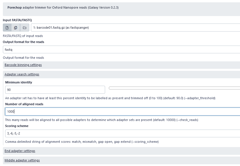
In order for the DNA to attach and translocate the nanopore and thereby enable sequencing, we add adapters to both fragments of our DNA (template and complement strand) in the library preparation step. Following sequencing, the adapters need to be removed from the raw sequencing data before further processing, as they are synthetic sequences. In the workflow, we will use Porechop with default setting to remove adaptors from the nanopore raw reads. If Porechop is running too slow, we can also use alternative programs such as cutadapt or trimmomatic.

Filtlong: Trimming short and bad quality reads

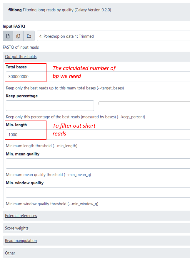
As a next step you are recommend subsetting and reducing the dataset with filtlong. This is not strictly necessary, but it will reduce the running time of the following steps and usually an average genome coverage of over 50 does not significantly improve the assembly in our experience. The coverage is defined by the number of reads that cover a given nucleotide. The genome coverage can be calculated by (number of total bp in reads)(genome length in bp) or alternatively (number of reads)(average read length in bp)*(genome length in bp). So to calculate the number of bp we need for a genome coverage of 50, we simply multiply the estimated genome size by 50, for example: 5 000 000 * 50 = 250 000 000. To be sure we can take 300 000 000 bp, which we then put in the setting “total bases” see image blow. Additionally, it is recommended to filter out shorter reads (<1000bp), since they are not helpful for the assembly.

Compare Raw vs Filtered Nanoplot Stats

We can get an overview of how our reads looked like after the filtering process by comparing the filtered with the raw Nanoplot stats.

Discussion 01

1. How much bp are discarded? Do you see a significant amount of data loss?
2. How does the quality of the data changed? Do you see increased N50 and read quality?

Solution

TBD

Assembly & Polishing

Flye: Assembling long-reads into whole genome

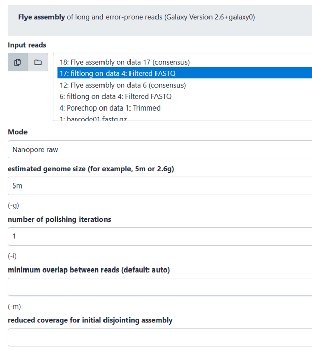
There is a wide range of different assembly tools, and you are free to choose which one you use. However, we advise you to consider the advantages and disadvantages of the tool you apply. Below, Flye was used as an example for the assembly of the trimmed and subsetted reads. Flye has been shown to have a high contig contiguity and accuracy, however it needs a lot or RAM usage and has a longer run time. So, if it runs to slow consider using a different assembly tool.

Quality check of assembly

After the assembly has finished running, we again need to check the quality. For that we can use three different measurements. We can first look at the assembly stats and the assembly graph.

Discussion 02 - Assembly stats

Open the “assembly_info” (see image) of flye.

1. What is the length of the assembly? Is it close to the estimated genome size?
2. How many contigs do we have?
3. What is the coverage of each contigs? Is it sufficient?

Solution

Discussion 03 - Assembly Graph Visualization with Bandage

For visualizing our assembly, we used the tool “Bandage image” with the default settings.

1. Look at the contigs visualization. How does your assembly graph looks like? Simple or tangled? Do you expect a circular or linear genome?
2. Can you spot the plasmids? What do you expect of a plasmid’s coverage compared to that of a genome?

Solution

Ideally, all reads are assembled into one genome (example 1), but the fewer pieces (=contigs) the assembly has, the better. Ideally these should also appear circular, as this illustrates a fit of all the reads into an entire genome. However, small contigs (as in example 2) could be plasmids, but could also have resulted from repeats in the genome, which could not be resolved by the assembler.

Medaka: Polising with Nanopore reads

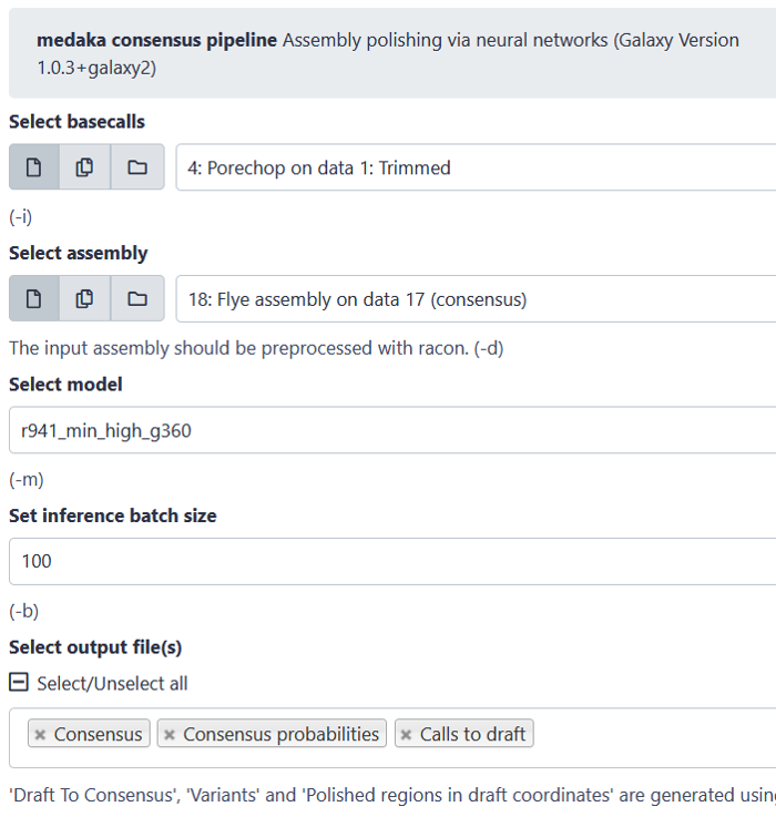
For polishing there are again several tools available. Be aware that some assembly pipelines already have the polishing included, while others don’t. Also, some polishing tools work better with specific assemblers. For the polishing example below, we applied the tool “medaka”, using the complete set of trimmed reads to polish our assembly. To check if the polished assembly has actually been improved compared to the unpolished assembly, we can again perform all the steps from (2).

Key Points

• Before assembling a genome, make sure to do a proper filtering and trimming to achieve the best assembly possible. There are various algorithm and tools to assemble and polish your genome. Decide which one suits your need.

• You can do a sanity check of your assembly by using prior knowledge such as: (1) expected genome size, (2) expected structure of the genome (circular or linear), (3) compare contigs length and depth distribution, and (4) make sense of the assembly graph. From this information, you can decide whether you need to add more depths (by re-sequencing) or do another run if the result is too fragmented.

Taxonomic Placement

Overview

Teaching: 10 min
Exercises: 10 min

Questions

• What is the taxonomic classification of my genome?

Objectives

• Assigning taxonomic classiffication to a newly assembled genomes using available tools.

Downloading the assembled sequence

We now have an assembled genome that we can analyze. Before moving forward, we would like to determine the lineage or taxonomic classification of this newly assembled genome. For that, we will need to first download the genome from galaxy.

1. Find the medaka consensus pipeline - Consensus result and click the Download icon (first from left) to save it to your computer. Hint: The file should be in .fasta format.

Taxonomic Placement with autoMLST

We will use autoMLST to get an overview which gives us the most similar organisms. Unfortunately, it is not available in the Galaxy server, so we must do the analysis in the autoMLST webserver.

1. Go to the autoMLST webserver
2. Choose the Placement (Fast) mode
3. Upload your genome sequence
4. Enter your email to get your result back
5. Click Submit job

Other tools to consider

There are also other bioinformatic tools for phylogenomic placement. Unfortunately, many of these tools are only available as a command line interface. Here are some tools to consider:

GTDB-tk

a toolkit for assigning objective taxonomic classifications to bacterial and archaeal genomes by placing the sequence to the GTDB tree database.

RefSeq_Masher

Find what NCBI RefSeq genomes match or are contained within your sequence data using Mash MinHash with a Mash sketch database of 54,925 NCBI RefSeq Genomes.

Discussion 01

Solution

TBD

Key Points

• Taxonomic placement of a newly assembled genome can be achieved by calculating nearest reference organism and placing the query genome into existing tree in the database. Such example of tools are autoMLST and GTDB.

Genome Annotation

Overview

Teaching: 10 min
Exercises: 30 min

Questions

• What genes are contained in my genome?

Objectives

• Assigning gene calls to sequence and annotate them with the known databases

Importing and editing Annotation workflow

Import genome annotation workflow:

1. In a new tab, open this link: https://usegalaxy.eu/u/matinnu/w/03annotation
2. On the top-right corner, click the + button (import workflow)
3. Click start using this workflow
4. Click on the name of the newly imported workflow (imported: 03_Annotation) and click Edit
5. Explore the workflow and make changes if necessary

When you are contempt with the workflow, click save. Next, we will run the analysis on the newly assembled genome (sample_02)

1. Click the “play” button on the top-right corner (Run Workflow)
2. If the workflow does not show in detailed view, click Expand to full workflow form
3. Set Send results to a new history to yes.
4. Change the history name to “03_Annotation_2021_sample02”.
5. On the 1: input dataset, select medaka consensus as the input.
6. Click Run Workflow on the top panel.

Prokka: rapid prokaryotic genome annotation

Prokka is a software tool to annotate bacterial, archaeal and viral genomes quickly and produce standards-compliant output files.

Discussion 01 - Prokka

1. What kind of output do you get from Prokka?
2. Which outputs can be used for subsequent analysis?

Solution

TBD

Busco:

Busco is a functional quality control based on evolutionarily-informed expectations of gene content of near-universal single-copy orthologs

Discussion 02 - Busco

1. What kind of output do you get from Busco?
2. How do you know if your genome is contaminated or incomplete?
3. What other tools can we use for quality checking our genome completeness and contamination?

Solution

TBD

Key Points

• Genome annotation starts by identifying genes and other functional elements (rRNA, tRNA, etc.) within the nucleotides. This is followed by comparison with databases of interest to predict the functions encoded in the genes.

Tools for analysing genomes

Overview

Teaching: 15 min
Exercises: 45 min

Questions

• How do I analyse my genome?

Objectives

• Assigning gene calls to sequence and annotate them with the known databases

The next steps are then to actually analyse the assembled genome. Dependent on your research questions and what you want to investigate, is a range of different tools that can help with the analysis. Here is a list of suggestions that might be of interest to you. You don’t have to do them all, choose the ones you find suitable to answer your research questions.

antiSMASH:

AnitSMASH stands for Antibiotics and Secondary Metabolites Analysis Shell and is used for the detection of secondary metabolites. To use AntiSMASH you first have to download your polished genome assembly from galaxy and then upload it to the AntiSMASH website. (https://antismash.secondarymetabolites.org/#!/start). After the it has finished the analysis job you will first be presented with a list of all detected secondary metabolite gene clusters, denoted as Region 1, Region 2 etc (labelled as number 5 in image). It will also tell you for each gene cluster the most similar known cluster detected in the MiBiG database, and the Similarity to that cluster. The Similarity is the percentage of genes within most similar known compound that have a significant BLAST hit to genes within the current region. So, the Similarity is NOT the same as the percentage identity that is an output of a Blast search. For more information on each Region, click on the number in the top (labeled as 2 in image). If you have experimental data on for example the bioactivity of your strain, try to match that to the potential compounds detected by AntiSMASH. For more information:

• https://docs.antismash.secondarymetabolites.org/understanding_output
• https://docs.antismash.secondarymetabolites.org/
• https://academic.oup.com/nar/article/39/suppl_2/W339/2507123
• https://academic.oup.com/nar/article/47/W1/W81/5481154

Discussion 01 - AntiSMASH

Solution

TBD

Abricate

ABRicate is a tool for the detection of antimicrobial and virulence genes. It is also available on Galaxy, so you don’t have to download your assembly for this. It uses different databases for example CARD to detect virulence genes in the genome. For more information: https://github.com/tseemann/abricate.
See below an example of default parameters with CARD database selected, an explanation of the output table and an example output.

Discussion 02 - Abricate

Solution

TBD

Blast

Lastly, you can also simply blast genes of interest against your assembled genome. For that you will first have to download the nucleotide or amino acid sequence of your gene of interest from NCBI (https://www.ncbi.nlm.nih.gov/). Then you can use nucleotide Blast or tblastn (dependent if you have the nt or aa of your gene of interest). Use the option align two or more sequences. Below an example for finding a gene of interest in your assembled genome.

Key Points

• Genome annotation starts by identifying genes and other functional elements (rRNA, tRNA, etc.) within the nucleotides. This is followed by comparison with databases of interest to predict the functions encoded in the genes.

Extra

Overview

Teaching: 15 min
Exercises: 0 min

Questions

• Using Command Line Tools for Bioinformatic Analysis

Objectives

• Getting a gist command line tools for a more flexibility in bioinformatic analysis

Where to start

A full genome assembly requires many curation steps, which is nicely summarized in the Genome Assembly Guide. When you have a nanopore only dataset, you can use trycycler to have a decent quality genomes through consensus approach. Nevertheless, the steps and tools can be complicated. Here, we wrap and simplifies the Trycycler into three steps using Snakemake.

Example: Semi-automated Trycycler Assembly via Snakemake

For Nanopore only assembly, Trycycler offer a better accuracy to generate consensus assembly (combining multiple assemblies of the same isolate). Rather than only using one assembler like we do (Flye), Trycycler can subsample our reads and build multiple assemblies using different algorithms, then make a consensus out of it. You can also find Trycycler in galaxy.eu toolbox, but as it is quite intensive, I prefer to run it on a local machine / server.

Installing and running a command line tools for a newcomer might seems daunting. Nevertheless, there are two popular workflow manager: Snakemake and Nextflow, which makes running various pipelines and installing dependencies easier. We have tried to make a prototype to semi-automate run Trycycler via Snakemake here: https://github.com/matinnuhamunada/trycycler_snakemake_wrapper.

The TAs will run it for you, but it is also quite easy to run it on your own when you have the time (and resources).

Key Points

• Galaxy might not have all the tools and version required to run your analysis. Having a skill to work with command line tools and other programming language give you flexibility in your research.